7.6 Parametric sequences

Section §7.5 shows how parametric equations can be realized as Myron tuple generators. Given a sequence of points, the plotter draws line segments between them. When they are close together, a continuously connected sequence of points provides a visual approximation of a curve. This section shows how collection generators are used to provide sequences of points to the plotter.

The following interpretations are used.

  • A point is determined by any composite value with 2 or 3 components. Complex numbers are naturally restricted to 2 components. Radial values are transformed to vectors as they are plotted.
  • A tuple of points provides a sequence of points.
  • A sequence that consists of exactly one point is drawn as a position vector. That is, a line is drawn from the origin to the point.
  • A set does not define a sequence. Elements of a set or set generator, whether sequences or points, are treated as separate graphical elements.

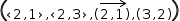
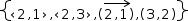
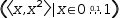
To illustrate the effects, consider the difference between ((2, 1)ʋ, (2, 3)ʋ, (2, 1)ɽ, (3, 2)), {((2, 1)ʋ, (2, 3)ʋ), ((2, 1)ɽ, (3, 2))} and {(2, 1)ʋ, (2, 3)ʋ, (2, 1)ɽ, (3, 2)}. The first expression contains a mixture of vector, radial and tuple-of-real values that define four points; they are drawn as three line segments. The second expression is a set of two tuples of points and is drawn as two line segments. The final expression is a set of four points and is drawn as four position vectors.

7.6.1 Simple Expression

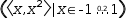
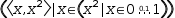
The simple plot displayed for an expression like x^2 is created by evaluating the expression at points with a constant step size over a range determined by the extent of the x axis. The step size and range can be specified explicitly by the generator ((x, x^2)ʋ|x∈-1, 1, 0.2) or implicitly be a generator with an axis domain ((x, x^2)ʋ|x∈𝕏). To show the power of this approach, the step size can be varied by replacing the domain with an exponential generator: ((x, x^2)ʋ|x∈(x^2|x∈0, 1, 0.1)). The bounds and increment of the generator can even be bound to constant expressions so that adjusters on the plot display can be used to vary them.

7.6.2 Segmented Circle

The parametric range control in Figure 7.11 draws part of a circle. A tuple of vectors generated over a range ((cos t, sin t)ʋ|t∈-ℼ, ℼ/2+0.1, 0.1) produces the same effect by providing a stream of x-y pairs when the tuple generator is evaluated.

A more elaborate example is given by a circle displayed as dashed lines. It can be plotted from

{((cos t, sin t)ʋ, (cos (t+0.1), sin (t+0.1))ʋ)|t∈-ℼ, ℼ+0.2, 0.2}.

(1)


If the tuple generator is placed in the body of a function, the length of the line segment can be bound to a parameter:

fʂ(w)→{((cos t, sin t)ʋ, (cos (t+w), sin (t+w))ʋ)|t∈-ℼ, ℼ+2⋅w, 2⋅w}.

(2)


Adding the function reference fʂ(d) along with a constant definition d→0.1 to the plotter allows the dash-length to be changed by a slider. Of course, expression (2) will have to be protected.

The dashed circle can also be displayed using nested generators, the inner for a dash and the outer for the sequence of dashes:

{((cos u, sin u)ʋ|u∈(t, t+d))|t∈-ℼ, ℼ, 2⋅d}

(3)


where d is the dash length as before.

7.6.3 Quadrature Diagram

The standard diagram for quadrature shows same-width rectangles whose height is given by a function. The diagram is used to show how the area under a curve can be approximated numerically by adding the areas of the rectangles. The diagram is given in Figure 7.12.
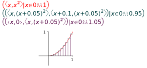
Figure 7.12 Quadrature

The plot in Figure 7.12 displays three separate expressions: two with disjoint line segments and one with joined line segments. The latter is the easiest, being given by ((x, x^2)ʋ|x∈0, 1, 0.1).

The horizontal lines are given by x-y pairs whose y value is the same:

(((x, (x+0.05)^2)ʋ, (x+0.1, (x+0.05)^2)ʋ)|x∈0, 0.95, 0.1).


The y value is the height of a rectangle and the x value locates the left and right sides.

The vertical lines are given by x-y pairs whose x value is the same:

(((x, (x+0.05)^2)ʋ, (x+0.1, (x+0.05)^2)ʋ)|x∈0, 0.95, 0.1).


The x value locates the vertical line and the y values take the line from the x-axis to the value of the function.